Basic Excel: Perbedaan revisi
| Baris 29: | Baris 29: | ||
!Session !!Content | !Session !!Content | ||
|- | |- | ||
| − | |align="center"| i || Welcome ceremony <br /> | + | |align="center"| i || Welcome ceremony <br /> Introductions |
| − | |||
|- | |- | ||
|align="center"| 1 || Principles of Data Management | |align="center"| 1 || Principles of Data Management | ||
| Baris 59: | Baris 58: | ||
=== Use of Excel === | === Use of Excel === | ||
This space is for your own notes. | This space is for your own notes. | ||
| − | |||
| − | |||
| − | |||
| − | |||
| − | |||
| − | |||
| − | |||
| − | |||
| − | |||
| − | |||
| − | |||
| − | |||
| − | |||
| − | |||
| − | |||
| − | |||
| − | |||
| − | |||
| − | |||
| − | |||
| − | |||
| − | |||
| − | |||
| − | |||
| − | |||
| − | |||
| − | |||
| − | |||
| − | |||
| − | |||
| − | |||
| − | |||
| − | |||
| − | |||
| − | |||
| − | |||
<br /> | <br /> | ||
<br /> | <br /> | ||
Revisi terkini pada 13 Maret 2014 14.30
Daftar isi
- 1 Building Beautiful Data in Basic Excel
- 1.1 Preface
- 1.2 Principles of Data Management
- 1.2.1 Use of Excel
- 1.2.2 Activity - examine an Excel workbook
- 1.2.3 Activity - inspect sample outputs
- 1.2.4 Objectives for good data management
- 1.2.5 Computer Management
- 1.3 Basic Excel Skills
- 1.3.1 Learning objectives
- 1.3.2 Introduction
- 1.3.3 Creating and saving a new workbook
- 1.3.4 Entering data into a cell by typing
- 1.3.5 Entering data by copying and pasting
- 1.3.6 Insert a column or a row
- 1.3.7 Moving items
- 1.3.8 Clearing the contents of a cell or cells
- 1.3.9 Deleting columns, rows, or cells
- 1.3.10 Cell data categories and formats
- 1.3.11 Formatting cells
- 1.3.12 Documentation
- 1.4 Cleaning Messy Data
- 1.5 Preparation of Useful Outputs
- 1.6 Appendices
Building Beautiful Data in Basic Excel
Preface
Course Aims
[To be completed]
Learning Objectives
After completing this workshop, you will:
- understand the principles of good data management
- be able to apply these principles to:
- creation of new Excel workbooks
- revision of existing Excel workbooks.
- be able to create and save a new Excel workbook and enter data
- be able to revise an existing Excel workbook to a form suitable for creation of pivot table reports
- be able to create and manipulate pivot tables.
Course Methodology
This workshop will be presented as a mixture of interactive discussion and 'hands-on' activities. Some of the activities will be demonstrated by your facilitator and will be projected on the large screen. Other activities will be conducted in pairs and small groups, using your computer, and you will be expected to follow the steps in your manual, asking a facilitator for assistance as required. In some cases, your manual will pose questions, and you will be expected to make notes in the manual in answer to those questions.
Microsoft Excel
This course has been based on Microsoft Excel 2010. If you use Excel 2007 or 2013 you may notice some small differences in the layout of menus, but most features should be very similar. Please advise your facilitator if you have difficulty completing any exercises due to version differences.
Course Outline/Timetable
| Session | Content |
|---|---|
| i | Welcome ceremony Introductions |
| 1 | Principles of Data Management |
| 2 | Principles of Data Management |
| 3 | Basic Excel Skills |
| 4 | Basic Excel Skills |
| Session | Content |
|---|---|
| 1 | Cleaning Messy Data |
| 2 | Cleaning Messy Data |
| 3 | Preparation of Useful Outputs |
| 4 | Wrap up/consolidation/debrief |
Principles of Data Management
Use of Excel
This space is for your own notes.
Activity - examine an Excel workbook
Learning objectives
After the completion of this activity, you will be able to:
- identify and open an Excel file
- navigate from one worksheet to another
- navigate within a single worksheet, using
- scroll bars
- menu system
- combinations of shortcut keys
- use zoom to view components of dataset
- select an individual cell, or a range of cells
- zoom to selection
- inspect the contents of a cell
- resize columns/rows
- apply/remove 'freeze panes'
- use freeze panes to keep selected rows and columns visible when scrolling around a worksheet
- apply/remove an autofilter
- use autofilter to inspect data.
Identify and open the file
Steps:
- Insert the USB stick provided into a USB port on your computer.
- Use Windows Explorer to browse to the 'Data' directory on the USB stick.
- Double-click on the faostatindo.xlsx file to open it in Excel.
The data in this Excel workbook was downloaded from FAOSTAT. The workbook contains multiple worksheets; the first worksheet shows the data exactly as downloaded. Your file should have opened on this first worksheet (Data asli).
Often, there is more than one way to do something. Here, we demonstrate three methods:
- Click on the appropriate worksheet tab
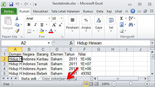
- Use shortcut keys
- Press the CTRL and Page Down keys together (CTRL+PAGE DOWN) to move to the next worksheet. (CTRL+PAGE UP will take you to the worksheet immediately preceding the current one.)
- Use the pop-up menu from the worksheet tab controls
- The worksheet tabs are useful when there are many worksheets in your workbook, and the tabs cannot all be viewed at once.
- Use the tabs to bring the desired worksheet into view, then click on its tab, as described above OR
- Hover the cursor over the righthand tab button, then right-click. A list of available worksheets will appear - click on the desired worksheet to move to it.
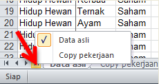
Practice moving from sheet to sheet using these techniques. Note the cursor positions on each worksheet. What happens if you move the cursor to a different cell (for example, by using the arrow keys, or by clicking on a different cell), and move to the other worksheet then back to this one?
Begin the exercise by placing your cursor in cell D42 of the Copy pekerjaan worksheet in the faostatindo.xlsx file.
Here are two ways to move the focus of your cursor (go) to a particular cell:
- Use the scroll bars to move the visible area of the screen around until you can see D42, then click on the cell.
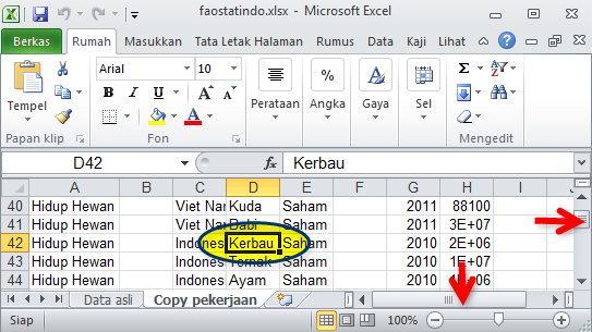
- 'D' refers to the column label (seen towards the top of the screen)
- '42' refers to the row number (visible at the left of the screen)
- Use the menu system to go to the desired cell directly.
- Make sure the 'Rumah' tab of the Ribbon has the focus (is selected).
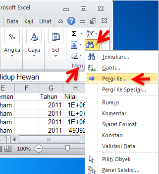
- Select 'Pergi Ke...' from the 'Temukan & Pilih' options on the 'Mengedit' section of the Ribbon.
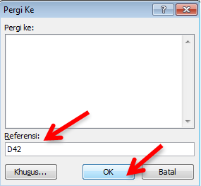
- Enter 'D42' (without quotes) in the 'Referensi' box, then click 'OK'.
Your task is to write your own description for the shortcut keys in the space provided. Sets of keystrokes that produce the same result have been grouped, so you will only need to write the description once.
| Keystrokes | The cell cursor moves to: |
|---|---|
| RIGHT ARROW | |
| TAB | |
| LEFT ARROW | |
| SHIFT+TAB | |
| UP ARROW | |
| DOWN ARROW | |
| HOME | |
| CTRL+HOME | |
| CTRL+END | |
| END then HOME | |
| PAGE UP | |
| PAGE DOWN | |
| CTRL+RIGHT ARROW | |
| END then RIGHT ARROW | |
| Double-click on the cell's right edge | |
| CTRL+LEFT ARROW | |
| END then LEFT ARROW | |
| Double-click on the cell's left edge | |
| CTRL+UP ARROW | |
| END then HOME | |
| Double-click on the cell's top edge | |
| CTRL+DOWN ARROW | |
| END then DOWN ARROW | |
| Double-click on the cell's bottom edge |
Viewing and zooming
Let us return to the Data asli worksheet.
- Do you remember the keyboard shortcut to do this?
Go to the end of the dataset.
- What are two ways to get there quickly, using keyboard shortcuts?
How many rows are there in this dataset (including the header row)?
When the last cell of data has the focus of your cursor, can you see the header row?
What happens if we try to see all of our data at once?
- Excel allows us to fill our viewing window with all material selected.
- This is particularly useful when projecting material onscreen.
- This may not be the best approach to review a larger dataset.
Selecting a range of cells
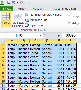
Let us select the cells in columns A to F, and from rows 1 to 10. The shorthand Excel notation for this is A1:F10, which tells Excel that we are interested in the the 'rectangle' of cells that has A1 as the top left corner, and F10 as the bottom right corner.
We could do this using the menu system, as previously described.
Alternatively, we could position the cursor in cell A1. Then, holding the SHIFT key, we click F10. The appropriate A1:F10 range should then be outlined and coloured, indicating that is has been selected.
We could use a number of methods to select our entire dataset at once. However, the quickest and easiest method is one that we have not yet used: CTRL+A.
- This method selects all cells in a contiguous data block.
- This is perfectly appropriate for the Data asli worksheet.
- Switch back to the Copy perkejaan worksheet, and see what happens if you use CTRL+A here:
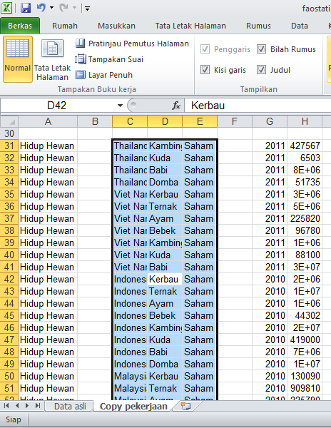
- Can you suggest a methods of selecting all occupied cells on this worksheet?
Zoom to selection
- Make sure that you are back on the Data asli worksheet.
- Select the 'Lihat' tab on the Ribbon.
- Choose 'Perbesar ke Seleksi' from the 'Perbesar' section of the Ribbon.
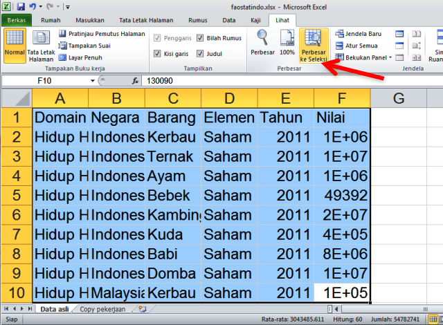
- Note that the effect of this varies, depending on the size of your viewing window, and the extent of your initial selection.
- Experiment with different selection sizes.
- Make sure to check what happens if you select, then view, the entire dataset in your viewing window!
- To return to 'normal' view, click '100%'.
- If you would prefer a differing amount of zoom, you can specify this using the 'Zoom' options.
Inspect the content of a cell
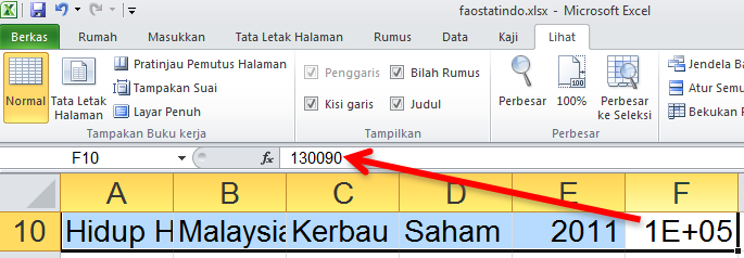
Consider the two images provided to you of the cell range A1:F10. The first was at 'normal' resolution; the second was zoomed so that the selection filled the viewable window.
In each case, the focus of the cursor was cell F10.
- How do you know this?
Inspect the apparent cell contents of F10:
- in the normal resolution version, it is 130090.
- in the zoomed version, it is 1E+05 (Excel's way of writing 1 x 10⁵)
The actual contents of the cell are the same (130090), in both cases:
The contents of the 'active' cell can always be seen in the Formula Bar.
Why are the (identical) cell contents displayed differently in these two examples?
- The size of the text relative to the cell is larger in the second example, and there is not enough room to display the six digits of the number, so scientific notation was used instead.
Resize columns/rows
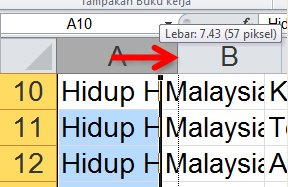
Individual rows or columns can be resized to reveal all their contents as follows:
- Select the desired row/column by clicking on its label.
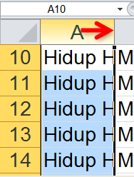
- Move the cursor to the righthand side of the column (or bottom of the row) label cell.
- When the colour of the highlighted label cell changes from orange to dark grey, and the cursor shape changes, the column or row can be resized.
The automatic resizing feature can be applied to multiple rows or columns at a time:
- Select all columns and all rows, by clicking in the intersection of the column and row labels.
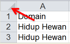
- The column and row labels will be grey (not orange).
- Move the cursor to the label cell of any column - it will change to orange, until the cursor reaches the edge of the cell, when it will return to grey. Double-click, and ALL the columns will be resized to fit their widest entry.
- Repeat this process for the rows (if necessary).
Freezing panes
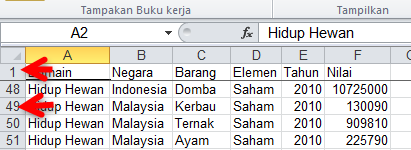
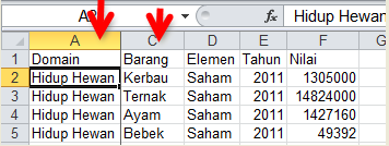
We have seen that navigating through a large dataset can mean that the header rows scroll off the top of the page. Excel has a feature that allow us to 'fix' desired rows and columns in place, allowing the rest of the dataset to scroll freely.
- Make sure that the 'Lihat' tab of the Ribbon is selected.
- Click on 'Bekukan Panel' in the Window section of the Ribbon.
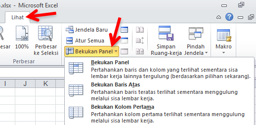
- Make your choice of type of freezing from the three options provided:
- Explore these options, using the scroll bars to move the 'unfrozen' portion of the spreadsheet around.
Freezing panes is very useful when the dataset is wide, or long, or both. This feature helps us to view and understand our data, and is one way to check for problems (for example, invalid or inconsistent data types, outliers, missing values). Another feature that is even more useful for checking for problems in the data is autofiltering.
Autofiltering
Autofilters are applied to a contiguous block of data, and are designed to be used on data that has a heading row.
- Although individual cells can be empty (blank), there must be NO completely blank rows or columns in the dataset.
Autofilters allow you to:
- find values in your dataset quickly
- identify groups used (for categorical data)
- identify minimum and maximum values (for numerical data)
- find outliers (extreme or aberrant values)
- locate missing values
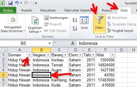
Apply an autofilter
- We will use the Data asli worksheet.
- Make sure that a single cell within the dataset is selected (has the focus).
- Go to the 'Data' tab of the Ribbon.
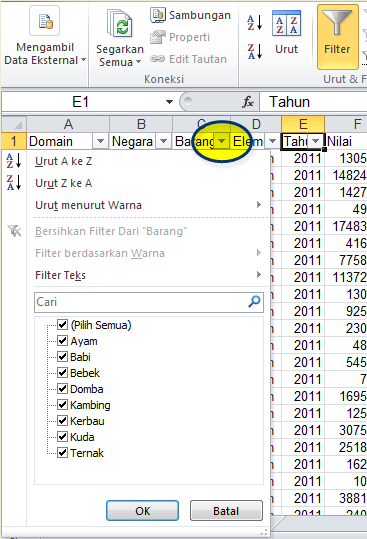
- Click on 'Filter' in the 'Urut & Filter' section of the Ribbon.
Examine the data
Each column heading now has a down arrow. Click on each of these in turn:
Use the autofilter to answer the following questions:
- Do any fields contain missing values?
- Which fields contain only one value?
- What type of field is 'Bilai'?
- What type of field is 'Tahun'?
- What are the categories for 'Negara'?
- What is the minimum value in the 'Nilai' field?
- What is the maximum value in the 'Nilai' field?
Now use a combination of filters to find the number of animals where:
- Negara = 'Indonesia'
- Barang = 'Ayam'
- Tahun = '2011'.
Which row of the dataset contained this record?
Note that more advanced filtering options are available, through both the 'Autofilter' and 'Advanced' tools; however, space and time limitations prevent us exploring these at this time.
Caution!
Before applying an autofilter, it is important to check that you will be applying the filter to the entire dataset of interest.
- An autofilter will be applied to the block of contiguous data in which the cursor is located when the autofilter is applied.
- Any blank (empty) rows or columns will restrict the scope of the autofilter to a subset of the data.
- This can have disastrous consequences if any of the autofilter's sorting options have been applied.
Sometimes, the presence of empty columns and/or rows is readily apparent (as it is in Copy pekerjaan). This is not always the case, and methods other than visual examination should be used to confirm that the autofilter will be applied to the entire dataset.
We recommend performing the following steps:
- Go to the cell that is the intersection of the last row with any data and the last column with any data.
- CTRL+END (or END then HOME)
- Note the identity of this cell.
- Return to the beginning of the dataset
- CTRL+HOME
- If this cell (A1) is not the leftmost cell of the header row, navigate to that cell.
- Do CTRL+RIGHT ARROW followed by CTRL+DOWN ARROW.
- Note the identify of this cell. Is it the same as that previously recorded? If so, there are no empty rows or columns in your dataset, and you can safely apply an autofilter.
This completes this activity. Please CLOSE the faostatindo.xlsx file, but do not save it.
Activity - inspect sample outputs
Learning objectives
After completing this activity, you will:
- be able to decide whether pivot tables and charts could be useful in your own work
- understand the underpinning data structure required for the construction of Pivot Tables and Charts
- be able to manipulate existing Pivot Tables and Charts to produce different outputs
- be able to provide input into development of suggested principles for good data and computer management.
Introduction to pivot tables and charts
A pivot table is a powerful tool for summarising, sorting, and presenting data. Using pivot tables, valuable summary information can be extracted from very large datasets without the need to understand or create formulae.
A pivot chart is an Excel chart based on the summarised pivot table data.
In this exercise, we will examine two pivot tables and a chart that are based on the data used in the previous activity.
Inspect the pivot tables and chart
Open the faostatpivot.xlsx file.
Go to the worksheet Pivot table 1.
The data source for a pivot table can be identified by:
- Selecting a cell (any cell) in the pivot table of interest.
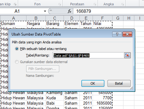
- Choosing 'Ganti Sumber Data' from the 'Opsi' tab of the 'Alat PivotTable' part of the ribbon, then selecting 'Gant Sumber Data...'.
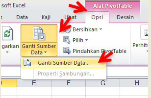
Check the data sources of pivot tables 1 and 2.
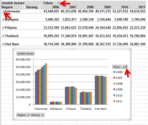
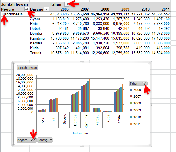
The facilitators will now demonstrate how changes to the type and amount of data displayed, and how it is summarised, can be made using the drop-down arrows on the pivot tables or chart, and by applying design options. Time will be provided for you to experiment with this yourself. In particular, notice how the chart reflects changes made to its associated table, and vice versa.
Two examples are provided, to get you started:
Objectives for good data management
General principles
This space is for your own notes.
Specific observations - pivot table requirements
This space is for your own notes.
Computer Management
This space is for your own notes.
Basic Excel Skills
Learning objectives
After completing this activity, you will:
- be able to apply the principles of good data management to design a simple data entry spreadsheet that is fit-for-purpose
- have mastered basic Excel data entry skills including:
- creating and saving a new Excel workbook
- entering information into a cell by typing
- copying and pasting data
- inserting a column or a row
- moving items
- clearing and deleting cells
- setting cell data categories and formats (text, number, date)
- setting cell appearance (font, highlight, styles, borders)
- insertion of comments
- insertion of illustrations.
Introduction
You will be creating an Excel workbook based on the data contained in the four pages of scanned data in the Resources section of the Appendices to this manual.
Suggested steps for the process of getting the scanned data into electronic Excel format are:
- Determine the required worksheet structure.
- This is the most important step. Plan to spend time on it.
- What metadata will be required, and where should it be stored?
- Create a new workbook, and save it.
- Enter the necessary metadata.
- Set up the data structures.
- Create the header row.
- Use of formatting (colour, fonts, shading) should be minimual.
- Apply any data formatting to assist clean data entry.
- Insert any explanatory comments in header fields.
- Create the header row.
- You may want to save the workbook at this time, with a different name, to act as a template for future (similar) data entry efforts.
- Enter data.
- Save your workbook frequently.
- How often - ask yourself how much work you could bear to lose.
- Wherever possible - use version control systems to avoid having to save multiple copies of files with different names on your computer.
- CTRL+S is a useful shortcut that can be used to save your workbook at any time.
The following material illustrates the skills that will be needed for the exercise, but is not based on the same material.
Please read through the material, and practise each skill using the exercise material. It is not necessary to perform each skill in the order shown here, but please make sure that you have worked through each skill.
If you used other skills in the exercise that have not been described here, please mention this to your facilitator so that they can be included in later editions of this manual.
Creating and saving a new workbook
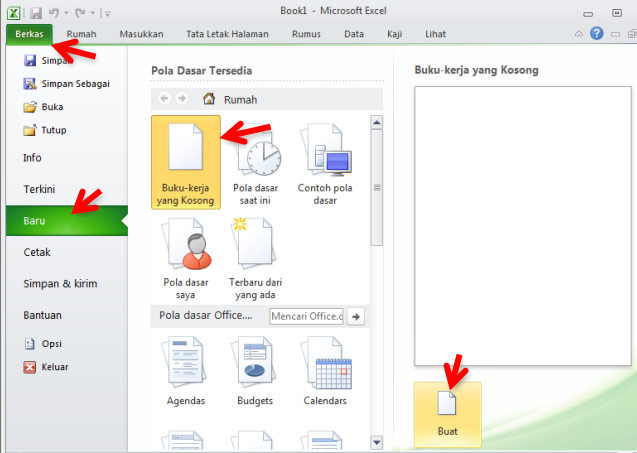
- Start Excel.
- Begin with a new (blank) workbook.
- Depending on your settings, the program may start by opening a copy of the last workbook you viewed, or (more likely) it will open with a blank workbook
- If a previously-opened workbook is displayed:
- Save the workbook to the desired location.
- For the purposes of this workshop, create a folder named 'Latihan' on your desktop.
- This can be done outside of Excel, in Windows Explorer, or as part of the file-saving process within Excel.
- Ask a facilitator if you need help with this step.
- Save your new workbook as 'Contoh1' in the 'Latihan' folder.
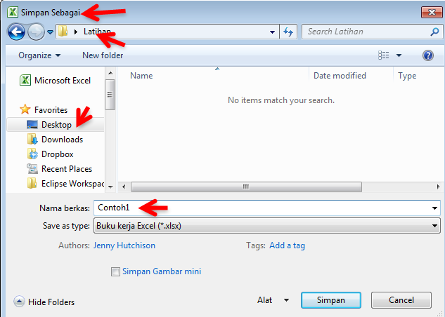
- For the purposes of this workshop, create a folder named 'Latihan' on your desktop.
Entering data into a cell by typing
Select the cell by clicking on it, then begin typing.
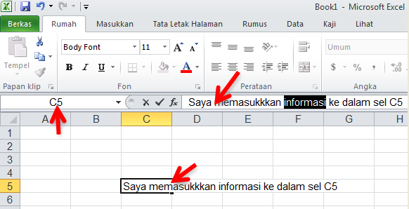
- The typed entry will appear both in the cell, and in the formula bar.
- The name box indicates the name of the active cell (if it has one - we will find out more about this later) or its column and row identifer.
Entering data by copying and pasting
Copying and pasting to a non-contiguous location
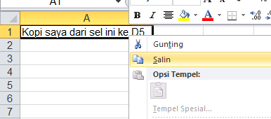
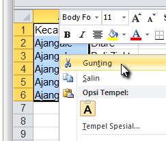
- Select the appropriate cell/s.
- Copy by:
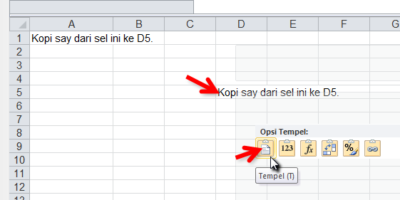
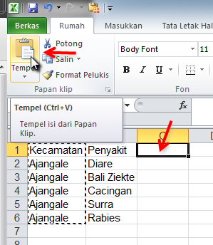
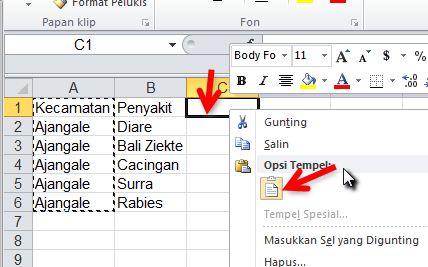
- Go to the (top lefthand corner of) desired location.
- Paste by:
Copying and pasting to contiguous cell/s (extent undefined)
Cells containing text only
- Select the desired cell.
- Move the cursor to the righthand edge of the cell until it changes shape to a '+'.
- Note that screenshots DO NOT show this shape change!
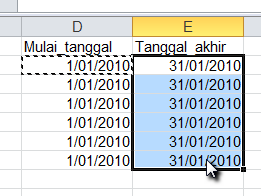
- Right click and DRAG the cursor to the desired extent of the copy range.
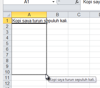
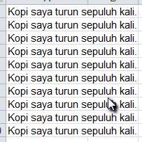
- Release the button. The cells will fill with the copied text:
Cells containing numbers, or numbers and text
When dragging a selection containing numbers to copy it, Excel will offer a choice between copying the selection exactly as it is, or incrementally increasing the numerical values as the data is copied. Two examples are provided below:
Cell with a number
- Select the desired cell.
- Move the cursor to the righthand edge of the cell until it changes shape to a '+'.
- Note that screenshots DO NOT show this shape change!
- Right click and DRAG the cursor to the desired extent of the copy range.
- Release the button. The cells will fill with the copied text, but there will be an option button at the bottom righthand corner of the selection:
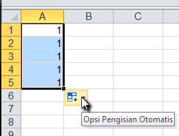
- If this is what you want, you can ignore this button. Otherwise, click on the down arrow to reveal options:
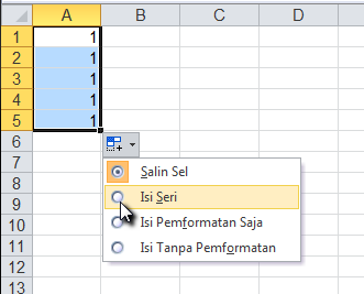
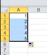
- Select 'Fill series' to fill the selection; by default, this will be done in 1 step increments:
Cell with numbers and text
This example shows how to use a selection containing more than one cell to define autofill behaviour:
- Select the desired cells.
- Move the cursor to the righthand edge of the bottom cell until it changes shape to a '+'.
- Note that screenshots DO NOT show this shape change!
- Right click and DRAG the cursor to the desired extent of the copy range. As you drag, you will be shown the suggested fill for the cells:
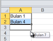
- Release the button. The cells will fill with the suggested items, but there will be an option button at the bottom righthand corner of the selection. In this case, 'Fill series' has been used as the default action:
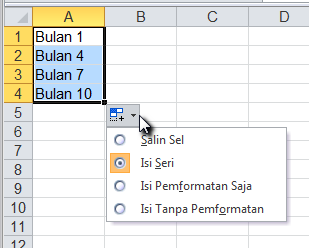
- If this is what you want, you can ignore the button and its options. Otherwise, make another choice from the options provided.
Copying and pasting to contiguous cell/s (extent already defined)
If you wish to copy a cell or cells to a region next to some existing data, proceed as follows:
- Select the cell or cells to be copied.
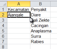
- Move the cursor to the bottom righthand corner of the cell.
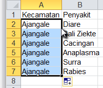
- When it changes in shape to a '+' sign, DOUBLE-CLICK.
- The data will be copied down the column to the extent of the data in the (longest) neighbouring columns.
Insert a column or a row
Column
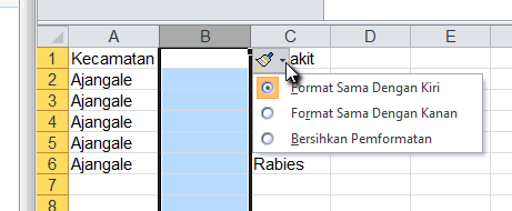
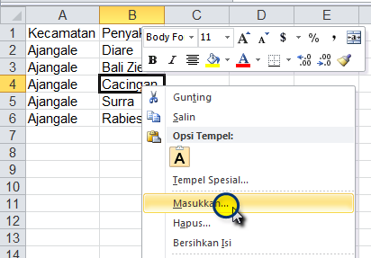
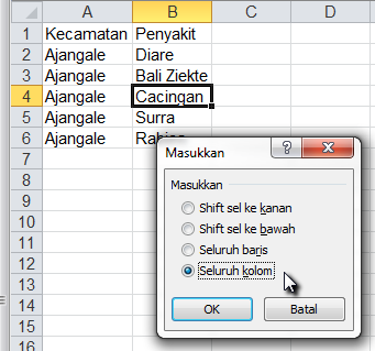
Here are two (similar) ways to do this:
- By selecting an entire column:
- By selecting a single cell:
Row
The steps for inserting a new row are the same as those shown for column above, with the exception that 'row' is used instead of 'column'.
New rows are inserted above the selected row or cells, and no formatting options are provided for the new row.
Moving items
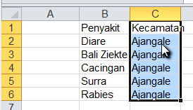
Drag
- Select the required cells.
- Move the cursor to the edge of the selection until it changes into an 'x' with four arrowheads.
- The changed cursor shape is not shown in the screenshots.
- Depress the left mouse button and, holding the button down, move the selection to the desired location.
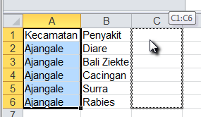
- Release the mouse button.
Cut and paste
- Select the appropriate cells.
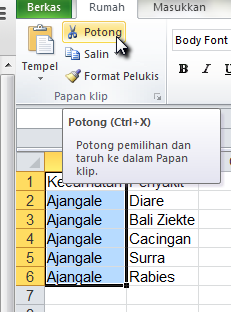
- 'Cut' the selection out, using any one of:
- 'Paste' the selection to the new location (which has been selected using its top lefthand corner), using any one of:
Clearing the contents of a cell or cells
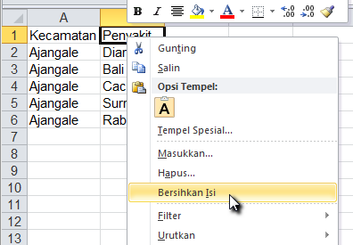
- Select the desired cell or cells
- Either:
Deleting columns, rows, or cells
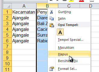
Columns
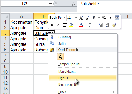
Here are two (similar) ways to do this:
- By selecting an entire column:
- By selecting a single cell:
Rows
The same approach described for columns is used to delete rows.
Cells or blocks of cells
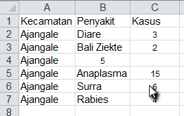
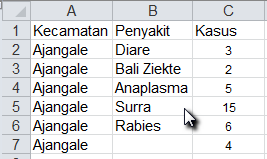
When the contents of a cell or block of cells is cleared, a 'gap' shows in the data - the surrounding data does not move.
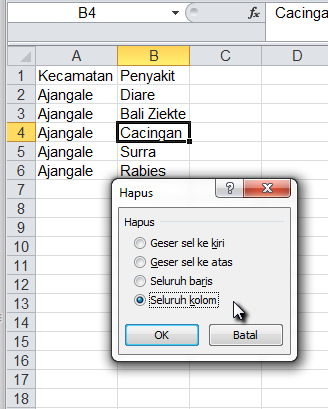
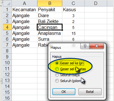
However, when a cell or block of cells is deleted, they are removed from the worksheet, and other cells must move into their space. You can choose to have cells from the right move into that space (shift cells left) or cells from below move up (shift cells up).
It is very important to think carefully about whether you want to clear or delete data. Moving cells out of position by deleting data can cause great problems with the integrity of the remaining data.
Shift cells left
This is the result of deleting a single cell (B4) using the 'Geser sel ke kiri' option:
Shift cells up
This is the result of deleting a single cell (B4) using the 'Geser sel ke atas' option:
Cell data categories and formats
Excel is a spreadsheet program. As such, it is particularly good at handling and displaying numbers.
Numbers can be formatted or presented in many ways. In the example below, the same number (40179) has been entered into the cells B2:B13, but different formats have been applied to each row:
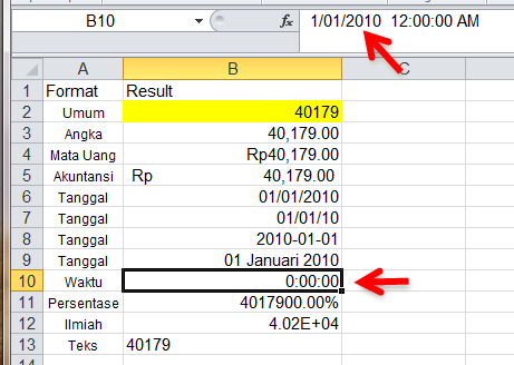
The number category of a cell or cells can be changed as follows:
- Select the cell or cells.
- Right click, then select 'Format sel' from the menu.
- Choose the appropriate category, then apply options within that category.
This is shown and discussed in more detail under the specific data types below.
Dates
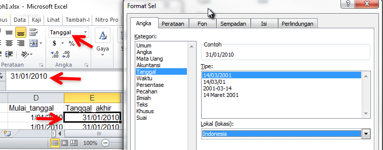
Excel understands the common date formats used in countries around the world, and when data is entered in a form that it thinks might be a date, it will treat the data as a date unless directed otherwise. This means that date data can be entered in a regular date format, and does not have to be converted to a number (Excel does this and stores that information internally). Although we rarely need to, we can force any number to become a date, as we showed for demonstration purposes in the example above.
There are many available date formats, but the ones displayed depend on the location selected:
Currency
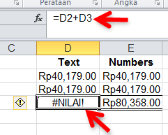
As a general rule, currency data should be entered as a simple number, and the appropriate currency or accounting format should be applied to the cells. In other words, currency data should NOT be entered as 'Rp40,179.00' as it will be seen as a text string, and it will not be possible to use the information in calculations or pivot tables.
In the example below, the data in cells D2:D3 were entered as 'Rp40,179.00'. In contrast, the data in cells E2:E3 were entered as 40179, and currency formatting applied so that the display appears identical to D2:D3 cells. However, because Excel interprets the data in cells D3:D3 as text, the formula in cell D4 does not work. The same formula (in cell E4) applied to cells E2 and E3 performs the calculation without problems.
Text
We have demonstrated above that it is important that numbers are recognised by Excel as numbers, so that they can be included in calculations. However, on occasions, it may be appropriate to apply a text format to cells that might contain numbers.
An example of this is the use of identifier codes that consist entirely of numbers and contain leading zeros. Such a numerical code is not intended for use in calculations. However, Excel will not know (without being told) that these numbers are special, and will treat them as numbers, and will remove the leading zeros. This can cause much confusion, as the (Excel-modified) identifier will not match the original data.
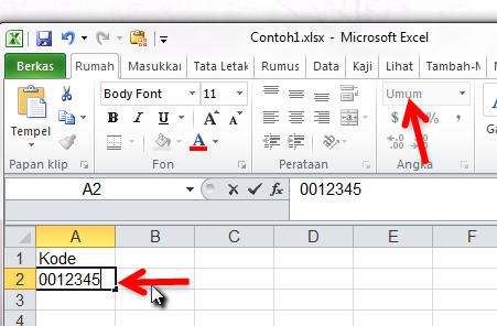
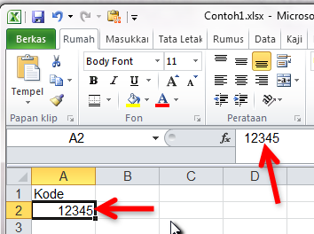
The example below show an identifer code '0012345' being entered into a cell that has the default 'umun' format. Perceiving the information to be a number, Excel removes the leading zeroes. The first figure shows the data in the process of being entered; the second figure shows the result after 'Enter' has been pressed.
Format cells as text
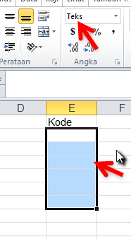
The solution to this problem is to apply the 'Teks' format to the range in which the data will be entered:
Note that it is not a good idea to apply formatting to an entire column - Excel then thinks that the data extends the length of the entire workbook, and file size can greatly increase.
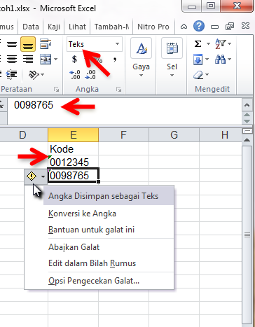
Now when (numerical) code data are entered, the entire string will be preserved.
As noted, these entries are now seen by Excel as text, and will not be used in any calculations.
Notice that Excel indicates that what it thinks is a number is being stored as text, and shows this by the small green triangle symbol on the lefthand edge of the cell. If the cell is selected, an warning exclamation mark is shown, with a down arrow. When expanded, this provides an explanation of the warning, and provides an option to convert the entry to a number.
Using the paintbrush to apply formats
Once the appropriate cell format has been chosen, it can easily and quickly be applied to other cells using the paintbrush:
- Select the cell that contains the desired format.
- From the 'Rumah' tab of the Ribbon, click on the paintbrush button.
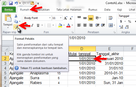
- Click once to apply the format to a single new cell.
- Click twice if you need to format a selection of cells.
- The cursor will change shape to a broad white cross, with a small paintbrush symbol, indicating it is ready to use to apply formats.
- Click on the target cell.
Formatting cells
We strongly recommend that only minimal formatting is applied to data entry worksheets. Formatting should be used to make the data entry requirements more understandable, or to differentiate data entry areas from other parts of the worksheet (e.g. instruction text, header rows).
Remember that the paintbrush can be used to apply a format from one cell to another cell, or range of cells.
Fonts
Many alterations in the appearance of a cell or group of cells can be made using the options available in the 'Fon' section of the 'Rumah' tab of the Ribbon.
Select the cell (or group of cells), then click the appropriate button. The 'Fon' tab of the 'Format Sel' dialog box will appear if the arrow at the bottom right of the 'Fon' section of the Ribbon is clicked:
Styles
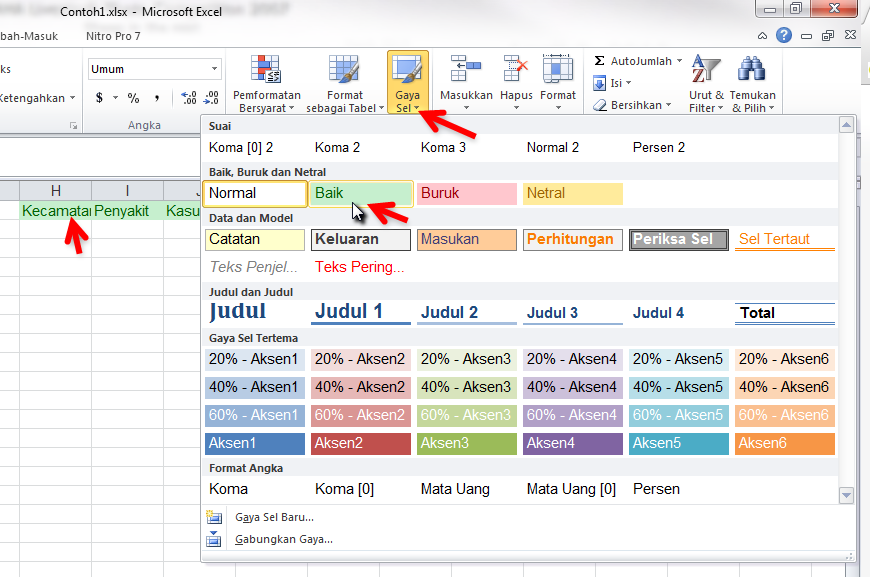
Excel contains some built-in formats called 'Styles' that can be accessed by clicking 'Gaya Sel' in the 'Gaya' section of the 'Rumah' tab of the Ribbon. It is possible to 'preview' the effect of the style by hovering the cursor over the style of choice - your selection will (temporarily) reflect that style, but it will not be permanent until the style is clicked:
Documentation
Explanations or instructions can be included to make it easier for others to understand your workbook and the data it contains.
Comments
Comments are particularly useful in headers.
- They can be used to explain the meaning of the field, or the type of data it should contain.
- They can be used to explain any abbreviations used for that data field.
Comments can be:
- added
- edited
- formatted
- moved or resized
- copied to other cells
- hidden or displayed
- deleted.
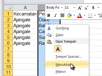
Insert a comment as follows:
- Select the cell to which the comment is to be applied
- Right click, and select 'Masukkan Komentar' from the menu.
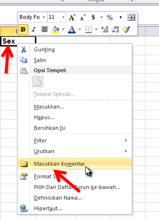
- Type the desired comment text in the box provided.
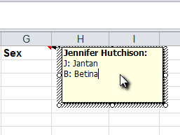
- Click outside of the comment box to save it.
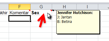
The presence of a comment is indicated by a small red triangle in the top righthand corner of the cell. A comment can be viewed by hovering the cursor on the cell; it is not necessary to select the cell:
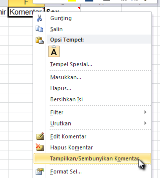
The menu displayed when a cell containing a comment is right-clicked provides options for editing, deleting, and showing or hiding the comment (this last option controls whether comments should always be visible, or only when the cursor hovered over the cell):
The default text in the comment (in the examples shown, this is 'Jennifer Hutchison:') is derived from the person or entity associated with this copy of Excel, and can be changed as follows:
- Select 'Opsi' from the 'Berkas' tab of the Ribbon.
- Choose 'Umum' from the categories in the left column.
- Edit the 'Nama pengguna' in the 'Personalisasikan salinan Microsoft Office anda' section:
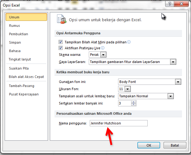
Note that changing this text will affect any new comments created, but will not change any comments already present in the workshop; these must be edited manually.
Special shapes
There are many special shapes or images that can be applied to your worksheet. We suggest that these are used sparingly, if at all.
Find these on the 'Masukkan' tab of the Ribbon, in the 'Illustrasi' section.
We will look at one example from the 'Bentuk' options - there are too many to explore in this workshop. If you are interested, and have the need, we suggest that you explore the other possibilities in your own time.
Insert and format a text box
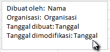
Text boxes can be useful for storing metadata that does not need to be uploaded to any other system, so does not need to be actual spreadsheet data.
- Select the text box from the 'Bentuk Dasar' section from the 'Bentuk' options.
- Position the cursor at the place on your worksheet that you want the top lefthand corner of the text box to be.
- Press the left mouse button. Holding the button down, drag the cursor to where you want the bottom righthand corner of the text box to be.
- Release the mouse button.
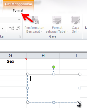
You should now have a box on your worksheet, ready to edit. You should also see a new Ribbon tab - 'Format', under 'Alat Menggambar'. If you do not see this option, or the cursor is not present as a vertical line flashing within the box, select the text box by clicking it:
Enter the desired text. When finished, click anywhere else in the spreadsheet other than the text box.
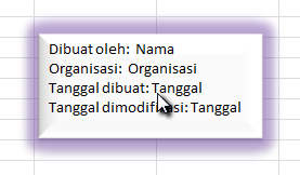
If you wish to modify the formatting of the text box or its contents:
- Select the text box.
- Click on the 'Format' tab of the Ribbon (under 'Alat Menggambar').
Cleaning Messy Data
Learning objectives
After completing this activity, you will be able to:
- determine whether an existing dataset has a structure that is suitable for basic analyses
- recommend a suitable structure for an existing (currently unsuitable) dataset
- identify the problems in a dataset that prevent its use for analysis
- manipulate such a dataset into a form suitable for analysis, applying existing skills, and using the following new skills:
- view multiple worksheets at the same time
- within a single instance of Excel
- using multiple instances of Excel (Excel 2010)
- copy a worksheet to the same, or another, workbook
- unmerging of cells
- text to columns
- find and replace.
- view multiple worksheets at the same time
Introduction
You may at times be asked to provide summary outputs or perform analyses based on data provided by someone else. This data will almost certainly not have been prepared for these purposes, and may not be in a format suitable for your needs. In this exercise, we will focus on manipulating existing data into a form that is appropriate for pivot table and chart creation. Pivot tables and charts are useful in their own right, but they also provide a good way to inspect the integrity of the underpinning data.
The data for this exercise is from the DAFF program of antibody titre sampling for avian influenza in the Sidrap and Pinrang Districts in June 2012. For the purposes of this exercise, you are told that you will be receiving additional very similar workbooks from other districts, and that the data must all be consolidated. You will be using the file DAFF_AI_SERO.xlsx
You will need to use many of the skills developed in the previous sessions. Additional skills that may be useful are outlined below; note that a number of techniques that are useful for cleaning and manipulating data involve more advanced Excel skills, and will be covered in the next workshop.
We recommend the following approach for working with a new dataset:
- Save a copy of the original data.
- Never make changes to the original dataset.
- Is there data on more than one worksheet in the workbook?
- Inspect each worksheet.
- Do not assume that an unnamed worksheet will be empty.
- Make sure you understand what you have been asked to do.
- What data will be needed to complete this task?
- Must all workbook data be processed?
- Does this workbook represent the complete task, or will additional (similar) workbooks be arriving?
- Outline the structure of the final structure that will be needed to complete the task.
- List the headers and data categories.
- Make a note of the problems or issues that make the original dataset unsuitable for immediate analysis, or that must be changed so that it fits your proposed structure. Look for:
- dataset not being contiguous (blank rows or columns separating components of the dataset)
- repeated heading row
- inappropriately formatted header row
- multiple header rows
- merged cells in header rows
- merged cells in columns
- repeated columns, or columns containing data that is not needed for the analyses
- this material does not need processing
- multiple pieces of information stored in a single column
- categorical data with inconsistent categories
- problem data
- some incorrect data will never be identified
- some incorrect data will only become obvious once the data summarisation has been completed (this will be the next exercise).
Note that the following material will not include all the skills that you are likely to use in manipulating your dataset. Many of the skills have been covered already (in earliers sessions), and you might already know some more advanced techniques that will be covered in the next workshop. However, if you find yourself using skills that are not listed here, please advise a facilitator so that they can be included in subsequent revisions of this material.
View multiple worksheets at the same time
It can be very helpful to view more than one worksheet at a time, particularly if you have a large screen, or multiple monitors.
Single instance of Excel
Make a copy of the DAFF_AI_SERO.xlsx workbook, naming it DAFF_AI_SERO_REVISED.xlsx (do this using 'Simpan Sebagai' from the 'Berkas' menu).
We now have only one workbook open - DAFF_AI_SERO_REVISED.xlsx, which contains four worksheets: SIDRAP, PINRANG, RESULT TEST, and an (empty) Sheet1. This workbook (probably) has only one 'window'. The 'window' is how we view or interact with Excel. It can be hard to understand what this means, at first, but the following example should help:
Inspect the 'Jendela' section of the 'Lihat' tab of the ribbon. A number of options ('Tampakan Berdampingan', 'Penyinkronan Penggulungan', and 'Reset Posisis Jendela') are not accessible (they are grey), because only one window is operating. Confirm this by clicking on 'Pindah Jendelah', and note that only one workbook is listed:
If we open another workbook through this instance of Excel (that is, using the 'Buka' or 'Terkini' options from the 'Berkas' tab of the ribbon), this opens a new window, which can be viewed at the same time as the original window.
Multiple workbooks - multiple windows
Open the original DAFF_AI_SERO.xlsx workbook as described. The sinlgle (active window) showing holds the most recently-opened workbook.
Notice how our ribbon options have changed:
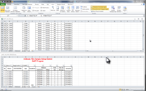
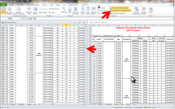
If we click the (now-active) 'Tampakan Berdampingan', we should find that two windows are displayed (each containing one of the workbooks), stacked horizontally:
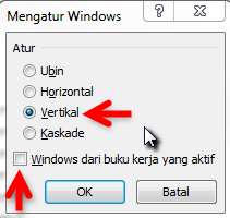
If we would prefer that our windows are displayed side-by-side, we can click 'Atur Semua' to start the 'Mengatur Windows' dialog box, and choose 'Vertikal' (making sure that the 'Windows dari buku kerja yang aktif' box is not checked):
Notice that the 'Penyinkronan Penggulungan' option is active - this means that the worksheets in the two windows will scroll simultaneously. Try this! In the example shown, they are not positioned at the same place in the file - to remedy this, just unclick the feature, scroll the sheets to the same place, then apply the feature again.
Multiple windows of the active workbook
Perhaps we would like to view different worksheets within the one workbook at the same time.
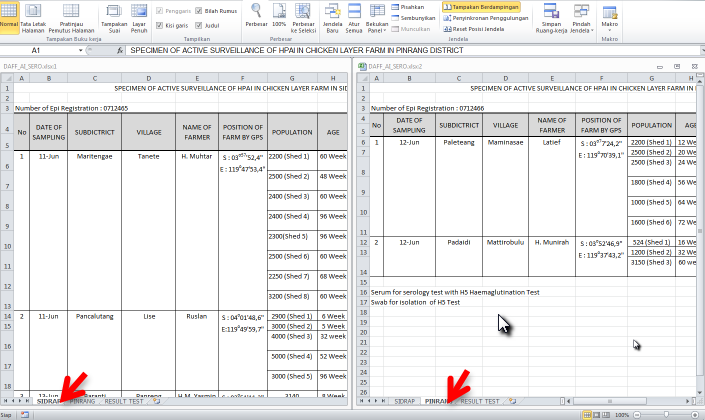
For the purposes of demonstration, we will leave the original workbook open, but will now focus our attention only on the DAFF_AI_SERO_REVISED.xlsx workbook. We want to have both the SIDRAP and PINRANG worksheets visible. To do this, we need to make a second window for the DAFF_AI_SERO_REVISED.xlsx workbook.
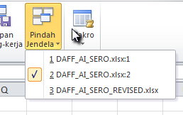
We do this by clicking 'Jendela Baru' (on the 'Jendela' section of the 'Lihat' tab of the Ribbon). At first, nothing seems to have happened. However, if we click 'Pindah Jendela', we see that two windows are listed for the DAFF_AI_SERO_REVISED.xlsx workbook:
Display the two windows of this workbook (leaving the other workbook in the background) by either of these two methods:
- Use 'Atur Semua'
- This method is particularly useful if you want to display more than two windows at once (we don't, in this case).
- Click 'Atur Semua'
- In the 'Mengatur Windows' dialog box, choose the desired configuration, and make sure to check the 'Windows dari buku kerja yang aktif' box.
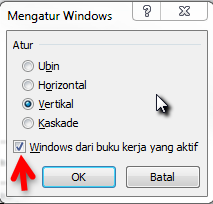
- Note that all windows of the active workbook would be opened - in this case, there are only two.
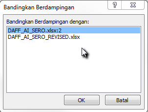
- Use 'Tampakan Berdampingan'
Both methods achieve the same result - two versions of the same workbook. We then choose the desired workbook sheets within each window, and uncheck the 'Penyinkronan Penggulungan' feature:
Window effects
It is important to realise that creating multiple windows of the same workbook does NOT create multiple, independent copies of the file. The windows are simply different ways of looking at the one object. A change made via one window will instantly be seen (is applied to) the same content in any other window that is 'looking' at the object.
Verify this for yourself! Change the style of the heading (row 1) of the SIDRAP worksheet, then navigate to that worksheet in the other window, and note that the same change has appeared there. Of course, these changes are not permanent until the file is saved; until then, they can be (individually) reversed using CTRL+Z.
Saving the Excel workspace
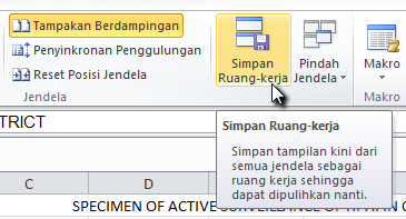
If you have opened a number of workbooks and windows, and have everything positioned just as you like it, it can be annoying to have to set everything up again, next time you work on the same material. However, this does not have to be a problem - you can use Excel's 'Simpan Ruang-kerja' feature to save the details of all your arrangements, so that next time you wish to work on the material, simply open the workspace file, and Excel will open all the workbooks and position everything exactly as it was when you saved the workspace. The file will be saved with a 'xlw' extension.
Make sure to save all the changes within the open workbooks before you save your workspace!
Multiple instances of Excel
If you are working with multiple monitors, you may wish to have an instance of Excel open on each monitor. The only way to do this with our previous example (using multiple windows within a single instance of Excel) would be to stretch the single instance across the multiple monitors. This is possible, but may not be convenient.
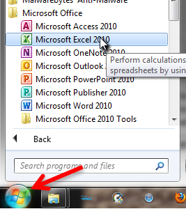
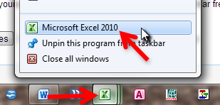
An alternative approach is to open multiple instances of Excel. This way, each instance gets its own Ribbon, and the opened files are independent of each other. Note than you cannot open the same file in multiple instances, unless you open a 'Read-Only' copy in the second and subsequent instances of Excel. In other words, changes can be made to only one open copy of a file at the same time.
You cannot start a new instance of Excel by opening an existing Excel file. Instead, you need to either:
Note that you can have multiple instances of Excel open, then have multiple windows within each instance of Excel.
Comparison: multiple vs single instances of Excel
You may find either, or both, of these options very useful. However, as you become a more advanced Excel user, note that it is very difficult to copy formulae from a workbooks in one instance of Excel to another (the result of the formula is pasted instead). There are no such problems when copying between workbooks opened in single instance of Excel.
Copy a worksheet to the same, or another, workbook
To make a copy of a worksheet, proceed as follows:
- Right-click on the worksheet tab, then select 'Pindahkan atau Salin...' from the resulting menu:
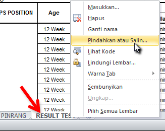
- Make sure that the 'Buat salin' box is checked on the 'Pindahkan atau Salin' dialog box (or the worksheet will be moved, not copied).
- To copy to another workbook, select the target workbook from the 'Ke buku' dropdown list.
- Select the place where the worksheet should be moved or copied to, then click 'OK':
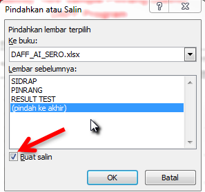
A copy of the worksheet will be created. By default, it will be named after the original, with a copy number in parentheses appended to the name.
Rename a worksheet
Either:
- right-click on the worksheet tab, then select 'Ganti nama' from the resulting menu OR
- double-click on the worksheet tab.
The black highlight means that the text is editable: type the desired name.
Unmerge cells
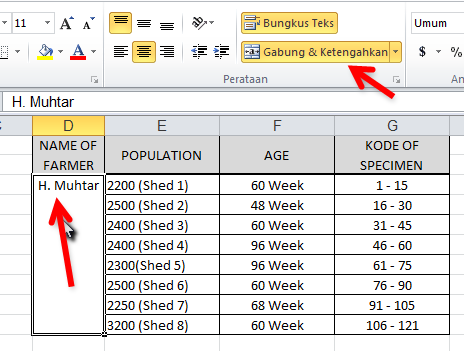
'Gabung & Ketengahkan' is often used in Excel to indicate that the item contained in the merged cell applies to all cells or columns captured by the merge. Often it is used simply for formatting purposes, as it can provide a visually-pleasing result.
However, we strongly advise against using 'Gabung & Ketengahkan', because it seriously limits the ability to use the data in any other way. (An alternative method of producing the same appearance as a merge, but without merging any cells, will be demonstrated in the advanced workshop). Pivot tables cannot be based on data that contains merged cells, so any merged data needs to be unmerged, and replaced with the appropriate contents, as demonstrated below:
In our example, merged cells have been used for two purposes:
- in the headings, cells from the first two rows have been merged to improve the appearance of the table
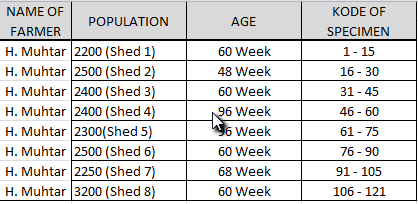
- in the first column, cells D3:D10 have been merged to indicate that the same farmer (H. Muhtar) is associated with each record:
To unmerge the cells, and refill the cells with the desired data:
- Select the merged cells.
- Click on 'Gabung & Ketengahkan' from the 'Perataan' section from the 'Rumah' tab of the Ribbon.
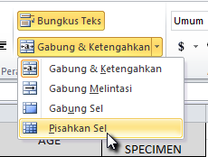
- Select 'Pisahkan Sel'. We can see that the cells have been unmerged, because we can see the cell gridlines.
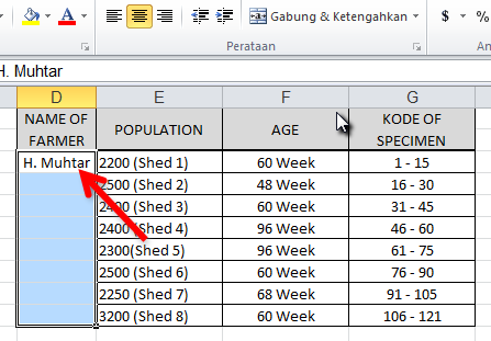
- The original content of the merged cells has been placed in the top lefthand cell - in this case, D3. Copy this data to the cells below:
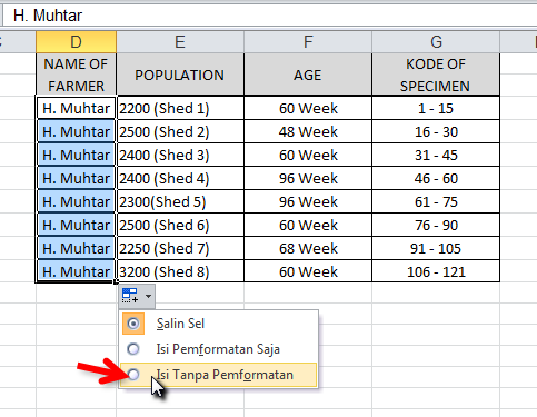
- Note that in this case, we elect to 'Isi Tanpa Pemformatan' to avoid copying the border formatting:
Text to columns
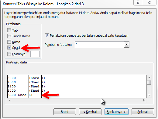
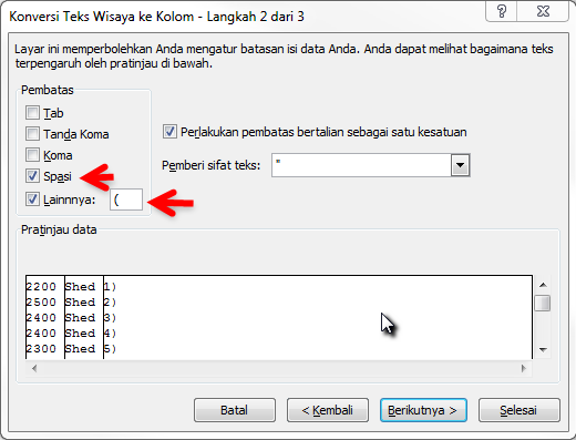
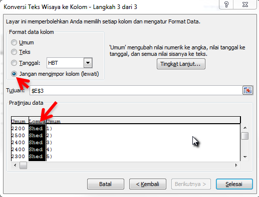
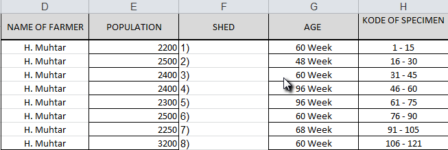
The 'Teks ke Kolom' feature can be used when more than one type of information is stored within a single cell. In our example below, we want to extract the number of birds that are in each shed, and the shed number. Cell E3 contains '2200 (Shed 1)'; we need the numbers 2200 and 1, each in its own cell. Using an automatic way to do this means that it can be done quickly and accurately.
We will use the 'Teks ke Kolom' wizard to split apart the data. The outputs will be placed in the cells on top of, and (if more than one) to right of the selected ones. In our case, we will have two pieces of output data. As we do not want the existing data in columns F and G to be overwritten, we must either INSERT enough columns to capture the split-out data, or move the data to the far right of the data region, so that nothing will be overwritten. We will demonstrate this second option.
Proceed as follows:
- Cut the existing column E, and paste it into column H:

- Select the cells that need to be split (here, they are H3:H10).
- From the 'Peralatan Data' section of the 'Data' tab of the Ribbon, click on 'Teks ke Kolom'.
- Check the 'Dibatasi' option on the first step of the wizard, then click 'Berikutnya'.
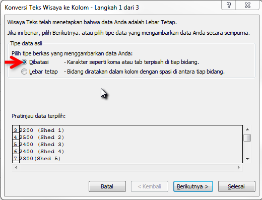
- We must now tell Excel what character/s should be used to split apart the cell contents.
- Click 'Berikunya' to move to the final step of the wizard.
- Each column in turn can be processed:
We are almost done:
We still need to:
- Name and format the header of column I.
- Name it 'Shed'.
- Apply the same formatting as the other header entries.
- Move columns H and I back to between the (current) D and F columns.
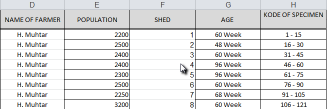
- Remove the ')' from the 'Shed' data.
Of these tasks, only the last will be demonstrated, as the skills for first two tasks have already been covered.
Find and replace
'Find and replace' can be used to replace an unwanted item with nothing, effectively removing the item. We will demonstrate this using our existing example:
We wish to remove all ')' from cells F3:F10.
Follow these steps:
- Select a range of cells that contains the data to be replaced (this saves Excel looking for, and replacing, data in other places).
- Select 'Temukan & Pilih' from the 'Mengedit' section of the 'Rumah' tab of the Ribbon, then choose 'Ganti' (or use CTRL+H).
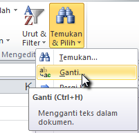
- In the 'Temukan dan Ganti' dialog box, type ')' in the 'Temukan apa:' box, and leave the 'Ganti dengan:' box empty.

- In this case, we choose to click 'Ganti Semua'.
- Excel makes the replacements, then tells us how many replacements were made. We click 'OK' to close this information message.
- If there has been a mistake: remember that previous actions can be reversed using CTRL+Z!
For your interest: Excel now sees the contents of cells F3:F10 as numbers - the data are oriented on the right hand side of the cell. In contrast, when the shed identifiers included the ')' character, the cells were seen as text, and the information was positioned at the left hand edge of the cells.
Preparation of Useful Outputs
Introduction
In an earlier exercise, we examined several pivot table outputs. In this exercise, we will learn how to create pivot tables and charts that can easily be updated with additional data as it becomes available. You will have opportunities to practise many of the Excel skills that you have already learned, and will master some additional techniques.
We will begin by creating a pivot table and chart together. We will then add additional data, and learn the steps needed to incorporate the new material into our existing output reports.
Learning objectives
After completing this exercise, you will be able to:
- understand the differences between a data range, a named range, and an Excel table
- name a range
- create an Excel table
- create an Excel pivot table from any of these (data range, named range, Excel table)
- determine whether a workbook contains hidden worksheets
- 'unhide' a worksheet
- 'hide' a worksheet
- add additional data to an Excel table
- update pivot tables with the additional data
- delete a worksheet.
Ranges, name ranges and tables
- Open the AIpivot.xlsx workbook.
- This is a subset of the data you were working with in the last activity - you should have ended up with something that looks like this.
- Take some time to quickly check over the data.
- You should always do this with every dataset you are given.
- Use the skills from previous sessions (for example, check the extent of the data, apply an autofilter).
- Are there any obvious issues with data integrity or the processing that has been done?
- Make two copies of this worksheet.
- Name the additional copies 'AIData2' and 'AIData3'.
Do you remember the exercise using faopivot.xlsx? In that exercise, the data source for the pivot table was simply a range of data. In our current exercise, we now have three ranges of data (which happen to be identical), one on each of three worksheets. Let us now name the range of data on AIData2, and make a table from the data on AIData3.
Naming a range
- Select the range to be named:
- Go the worksheet 'AIData2'.
- Select the data.
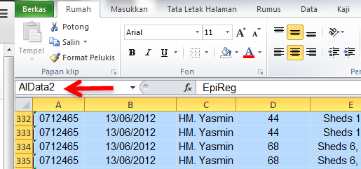
- Type the name 'AIData2' into the name box, then press ENTER.
Checking named ranges
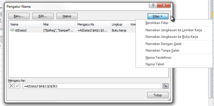
- From the 'Nama Terdefinisi' section of the 'Rumus' tab of the Ribbon, click 'Pengatur Nama':
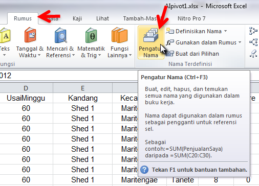
- From the worksheet's name box, click the down arrow to reveal a list of existing named ranges. Clicking on any one of these will take you to (and select) the range, even if it is on another worksheet.

Insert an Excel table
- Select the range to be turned into a table:
- Go the worksheet 'AIData3'.
- Select the data.
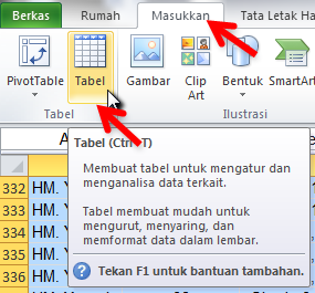
- Click on 'Tabel' from the 'Tabel' section of the 'Masukkan' tab of the Ribbon.
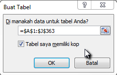
- Make sure that the 'Tabel saya memiliki kop' box is checked.
- Take the opportunity to look closely at the result:

- Notice:
- A new tab on the Ribbon, which will only be visible when the table is selected ('Alat Tabel'/'Desain')
- The opportunity to give this table a name - by default, this is Tabel1. Change this to AIData3.
- The format of the data range has been changed, to help show that it is a table.
- An autofilter has been applied.
- The top (header) row is frozen.
- Notice:
Insert a pivot table
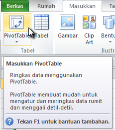
Pivot tables can be created from two places, both of which lead to the same 'Buat PivotTable' dialog box:
- 'PivotTable'form the 'Tabel' section of the 'Masukkan' tab of the Ribbon
- 'Rinkas dengan TabelPivot' from the 'Alat' section of the 'Alat Tabel/Desain' tab of the Ribbon (visible only when an Excel table is selected).
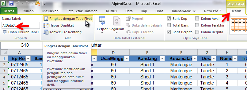
The default value for the 'Tabel/Rentang' box in the 'Buat PivotTable' dialog box will be the (contiguous) data range or table (if it was part of one) of the cell that was selected when the dialog box was launched. This entry can be changed, either by inserting a named range (in this case, we could use AIData2 or AIData3) or by choosing a new range.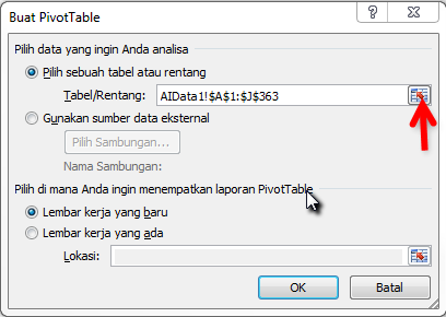
We will create our first pivot table using the unnamed data range on the AIData1 worksheet. We elect to place the pivot table on a new worksheet:
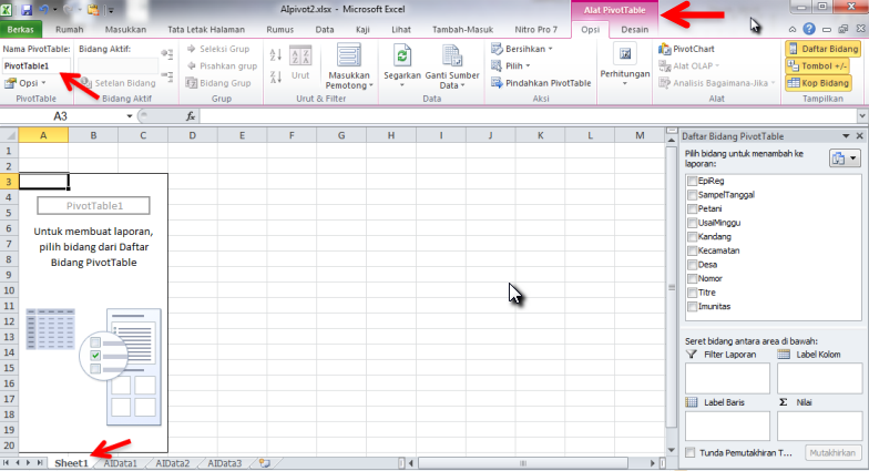
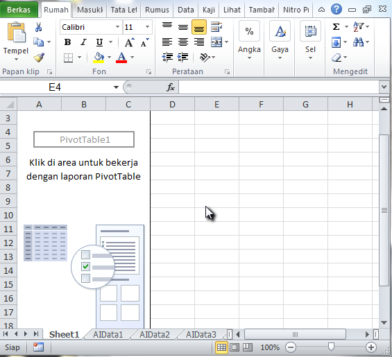
Note that although our pivot table has been created based on the data selected, we see only a 'placeholder' for it, as we have not yet specified its structure. We can see this by removing the focus from the pivot table by selecting a cell that is not on the pivot table (for example, E4). We see that the 'Alat PivotTable' tabs disappear from the Ribbon, and our 'Daftar Bidang PivotTable' dialog box also disappears. We are left with the pivot table 'shell':
Specify pivot table structure
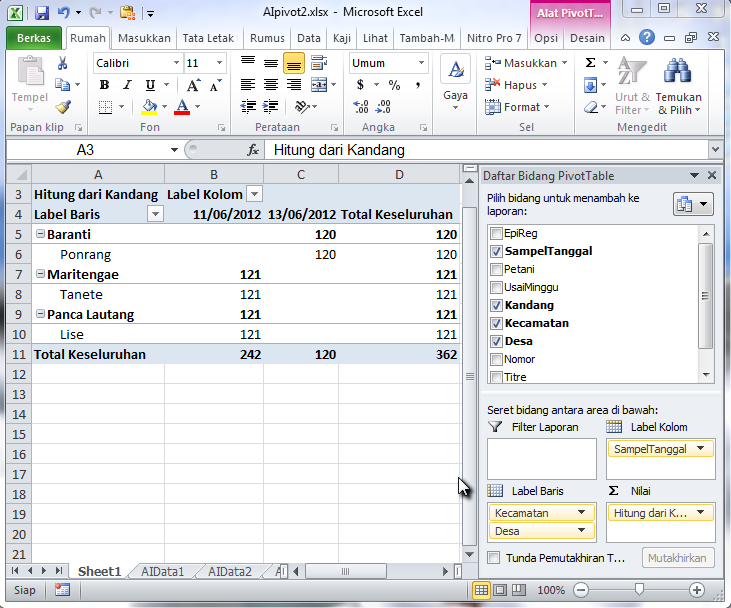
Our objective for our first pivot table is to determine how many samples were tested each day, by subdistrict and village. Note that Excel will automatically attempt to sum outputs that it sees as numeric, but will count items if a text field is put into the 'Nilai' box. As we wish to count the numbers of samples, we will use any of the fields containing text in 'Nilai' (please experiment to see the effects of using different choices). Move the fields by dragging:
To keep matters organised, please rename this worksheet 'PivotTable1', and move it to be positioned after AIData3 in the workbook (drag its tab).
Create additional pivot tables
Create two additional pivot tables as follows:
PivotTable2
- Base this one on the named range 'AIData2'.
- Place it on a separate worksheet.
- Use it to determine how many seropositive and seronegative samples there were in each sub-district.
- Name the worksheet PivotTable2, and move it to the end of the workbook.
PivotTable3
- Base this one on the table named 'AIData3'.
- Place it on a separate worksheet.
- Use it to determine how many seropositive and seronegative samples there were for each antibody titre result.
- Name the worksheet PivotTable3, and move it to the end of the workbook.
Incorporate additional data
We will now add additional data to our datasets. This data is on hidden worksheet that must be 'unhidden' so that we can take copies of its data.
Unhide a worksheet
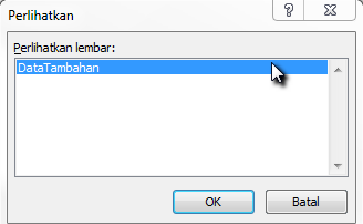
Check for hidden worksheets by right-clicking on (any) worksheet tab. If hidden worksheets are present in the workbook, the 'Ungkap...' option is available:
In this case, we find only one hidden worksheet listed, so we select it:
Hide a worksheet
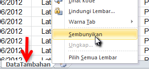
To hide a worksheet, right-click on its tab, then select 'Sembunyikan' (note that we do not need to do this here):
Add the data
Copy all the data on the 'DataTambahan' worksheet.
Paste these data at the end of each dataset on worksheets AIData1, AIData2, and AIData3. Do not leave any blank rows between the copied and the original data. Delete the (extra) copied header row (row 364).
The pasted data on worksheets AIData1 and AIData2 should both look like this:
In contast, the pasted AIData3 worksheet looks different:
Refresh a pivot table
Refreshing a pivot table means that Excel goes back to the data source specified for the pivot table, then rebuilds the pivot table using these data. If the content (or extent) of the data source has changed, this will be reflected in the pivot table.
Refresh a pivot table as follows:
- Select the pivot table.
- The 'Alat PivotTable' tab of the Ribbon becomes visible.
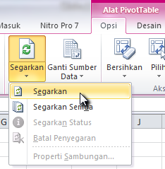
- Select 'Segarkan' from 'Segarkan' on the 'Opsi' tab:
Do this for each of the three pivot tables. What do you find?
Effect of data source
You should have found that only PivotTable3 incorporated the additional data. Before reading further, can you explain why?
To refresh your memory, check the data source of each of your pivot tables:
PivotTable1: AIData1!$A$1:$J$363
PivotTable2: AIData2
PivotTable3: AIData3
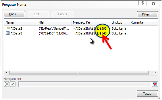
Now check the data ranges that comprise AIData2 and AIData3 (we covered that earlier in this session):
Only the Excel table automatically incorporated the additional data into its definition. This is the key reason for basing pivot tables and charts on an Excel table - any data added to the table will automatically be added to the scope of the table, and will appear in the pivot table once it has been refreshed.
Change pivot table data source
Change the data source of PivotTable1 and PivotTable2. Set the new data source to be AIData3.
Select and delete multiple worksheets
For housekeeping purposes, delete worksheets AIData2 and DataTambahan:
- Select multiple worksheets at once by holding down the CTRL key as the worksheet tabs are clicked.
- Right-click on one of the selected worksheet tabs, then click 'Hapus' from the menu.
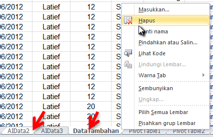
Finally, save the workbook.
Inspect and assess the data
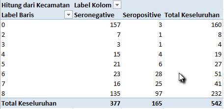
PivotTable3 shows some interesting results:
Your task is now to work out what is happening here. Are there errors in the data?
Your training has provided you with the skills necessary to complete this task. You may need to:
- create one (or more) additional pivot tables
- use autofilters to focus on the problem data records
- inspect cell contents.
Clue: how is the sample coded as being seropositive or seronegative? How does this differ between the original and additional datasets?
Describe the problem in your own words:
This space is for your own notes.
How would you fix the problem in this workbook?
This space is for your own notes.
How would you prevent the problem from happening again (in other situations, with other data)?
This space is for your own notes.
Appendices
Resources
Basic Excel Skills
Data Pelayanan Kesehatan Hewan (Keswan) 1
Data Pelayanan Kesehatan Hewan (Keswan) 2
Data Pelayanan Kesehatan Hewan (Keswan) 3
Data Pelayanan Kesehatan Hewan (Keswan) 4
Reference
| ID | Keystrokes | The cell cursor moves to: |
|---|---|---|
| A | RIGHT ARROW | One cell to the right. |
| A | TAB | |
| B | LEFT ARROW | One cell to the left. |
| B | SHIFT+TAB | |
| C | UP ARROW | One cell up. |
| D | DOWN ARROW | One cell down. |
| E | HOME | The beginning of the same row (column A). |
| F | CTRL+HOME | The beginning of the worksheet (cell A1). |
| G | CTRL+END | The last cell of the worksheet (lowest used row of rightmost used column). |
| G | END then HOME | |
| H | PAGE UP | One screen up (in the same column). |
| I | PAGE DOWN | One screen down (in the same column). |
| J | CTRL+RIGHT ARROW | The rightmost edge of the current data region (block of contiguous cells) in the same row. |
| J | END then RIGHT ARROW | |
| J | Double-click on the cell's right edge | |
| K | CTRL+LEFT ARROW | The leftmost edge of the current data region (block of contiguous cells) in the same row. |
| K | END then LEFT ARROW | |
| K | Double-click on the cell's left edge | |
| L | CTRL+UP ARROW | Top edge of the current data region (block of contiguous cells) in the same column. |
| L | END then HOME | |
| L | Double-click on the cell's top edge | |
| M | CTRL+DOWN ARROW | Bottom edge of the current data region (block of contiguous cells) in the same column. |
| M | END then DOWN ARROW | |
| M | Double-click on the cell's bottom edge |

