Notes: Key concepts for Sampling
Daftar isi
Notes: Key concepts for sampling
Sampling
Imagine we would like to know what proportion of cattle in a district is sero-positive to brucellosis.
We could test all the cattle in the district for brucellosis. When every animal in the population is measured this is called a census. Most of the time it is too difficult to do a census. Instead we test a small number of animals from the population (known as a sample).
Provided the sample is representative of the population then the results of the sample can be applied to the population. If the sample had 20% sero-prevalence then we may conclude that 20% of the entire district population will be positive.
How well the sample results reflect the true state in the population depends on bias and sampling variability.
The term bias is used to describe the situation where the results from a sample do not reflect what is occurring in the population. The reason is often due to poor selection of individuals into the sample. So we must think about how the sample might be selected to ensure that the animals chosen in the sample are representative of the target population.
For example, imagine if you sampled only the largest, most healthy, young animals for testing. If all these animals test negative for brucellosis, can you assume the district prevalence of brucellosis is 0%? The answer is no. There may be other animals in the population (older sick animals) that are infected and the results from the sample of healthy, young animals do not represent the entire population. This poor sample selection may lead to a biased study result. It would be better to select a representative sample of cattle. This would mean that some old and some young animals are included in the sample.
Sampling variability means that each time a sample is taken from a population; the results of the sample will differ. For example, assume we took five separate samples, each of 20 cattle from the district. Also assume the true but unknown sero-prevalence of brucellosis was 20%. We would get several different estimates of sero-prevalence from our five samples such as 21%, 18%, 22%, 25% and 14%. None of them are correct, but all are somewhat close to 20%. Using statistics we can improve our estimate of from just one sample by showing how confident we are that the estimate is correct.
If you use representative sampling and account for sampling variability you can get virtually the same information from a sample as a census at a much lower cost. For example, we could take a representative sample and using statistics show that the sero-prevalence estimate is 19% and that we are very confident that the true value of the sero-prevalence is between 17% and 23%. If an estimate that may vary by as much as 3% either way is acceptable, then you can save a lot of money by sampling instead of taking a census. However, the use of statistics is essential to do this. We will show you how to do these sorts of statistics correctly in this course.
Datasets and variables
Imagine we measure liveweight (kilograms) of a large number of adult Bali cattle. The individual liveweight measures can be entered into an Excel column (one weight record per row with a column heading called weight). In epidemiology and statistics we can call this column of weight measures a variable with the variable-name being weight.
The same dataset might include additional variables measured on the same animals. For example we might record an ear-tag number or some other form of animal identification (animal id), the sex of the animal may be recorded as bull, steer, female (sex) and the age of the animal may be recorded in broad categories such as calf, weaner, adult (age class). Some of these variables may contain numeric data (ear tag number and liveweight) and others may contain text records. Each row will contain records from one animal. Together these variables may form one dataset or set of data.
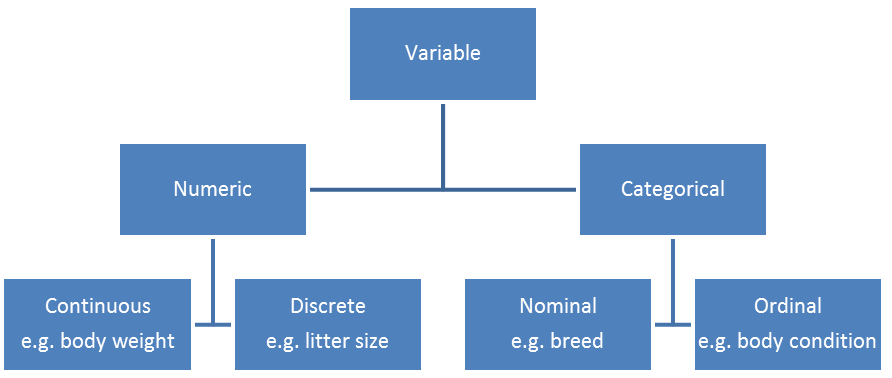
The different variables (e.g. age class, weight, sex, animal ID) can be classified in order for one to understand them better. Variables can be either numerical or categorical.
Numerical variables are measured in real numbers, and can be either continuous or discrete. Continuous variables can be any number between a set of real numbers, for example weight. Discrete variables can only be a particular number (usually a count), for example the size of a litter.
Categorical variables can be either nominal or ordinal. A nominal variable has no measurement value - they are "named" values, for example sex. Ordinal variables have a particular order to them, such as an age class (calf, weaner and adult), but there isn't a consistent interval between them. See Figure 1.
Figure 1: Types of variables that can be used in data analysis
Distributions
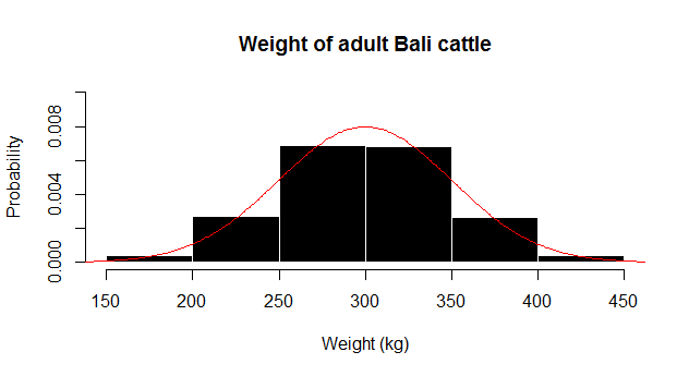
Our dataset contains many rows recording the liveweight (kg) of adult Bali cattle. A histogram is a common way to plot such data and one is shown in Figure 2.
Figure 2: A probability distribution function (red-line) and histogram (black bars) of adult Bali cattle liveweights.
The histogram provides a probability[1] on the vertical axis. Liveweight measures are sorted and classified into several bins on the horizontal axis. In this case the bins are all 50kg wide (150-200, 201-250, 251-300 and so on).
The histogram shows the probability that animals from our sample were in each liveweight bin. The histogram shows the pattern of spread of liveweight measures in our sample or the distribution of our sample. We can see that the smallest weights were between 150-200kg, the most common weight was somewhere between 250-300kg and the highest weight was between 400-450kg. Also it can be seen that lower and higher weights are rare.
The red line shows a theoretical normal distribution. Normal distributions occur commonly in nature and have a single central peak with a symmetrical shape. Normal distributions are often described as a bell curve because of their shape. The histogram of our liveweight sample tells us that our data are normally distributed because it looks like this typical bell shaped normal curve.
In statistics we can use two simple summary measures to describe a normal distribution: the mean (centre of the distribution) and the variance or standard deviation (a measure of the spread around the mean).
Many statistics are based on the normal distribution. If you take large enough samples when you are sampling and you are estimating a common statistic, then there are a lot of statistical approaches available to you since you can assume your statistic is normally distributed. We will use this assumption later.
An important thing to realise is that there are many different types of distributions besides the normal distribution. Several common distributions used in the analysis of animal health data are the binomial distribution, the Poisson distribution, the chi-squared distribution and the logistic distribution.
- ↑ Probability is a measure of how likely something is to occur. Probabilities are given a value between 0 (will not occur) and 1 (will definitely happen). So if probability (p) =0.5, then it is just as likely to occur as not to occur. If p=0.999 it is very likely to occur. If p=0.001 it is not very likely to occur.


